

Unit Step Function Laplace Transform
eight.4: The Unit Footstep Office
- Page ID
- 9435
In the next department we'll consider initial value issues
\[ay''+past'+cy=f(t),\quad y(0)=k_0,\quad y'(0)=k_1,\nonumber \]
where \(a\), \(b\), and \(c\) are constants and \(f\) is piecewise continuous. In this department we'll develop procedures for using the table of Laplace transforms to find Laplace transforms of piecewise continuous functions, and to find the piecewise continuous inverses of Laplace transforms.
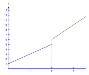
Use the table of Laplace transforms to notice the Laplace transform of
\[\label{eq:8.4.i} f(t)=\left\{\begin{assortment}{cl} 2t+1,&0\le t<2,\\[4pt]3t,&t\ge2 \stop{array}\right.\]
(Figure 8.iv.one ).
Solution
Since the formula for \(f\) changes at \(t=2\), nosotros write
\[\label{eq:8.four.ii} \begin{array}{ll} {\cal L}(f)&= \int_0^\infty e^{-st}f(t)\,dt \\{} &= \int_0^2 e^{-st}(2t+ane)\,dt+\int_2^\infty e^{-st}(3t)\,dt. \terminate{array}\]
To relate the first term to a Laplace transform, we add and subtract
\[\int_2^\infty e^{-st}(2t+one)\,dt \nonumber\]
in Equation \ref{eq:8.iv.two} to obtain
\[\label{eq:8.iv.3} \begin{array}{ll} {\cal L}(f) &{= \int_0^\infty due east^{-st}(2t+1)\,dt+ \int_2^\infty e^{-st}(3t-2t-one)\,dt }\\ {}&= \int_0^\infty e^{-st}(2t+ane)\,dt+ \int_2^\infty due east^{-st}(t-1)\,dt \\{} &{={\cal L}(2t+1) + \int_2^\infty e^{-st}(t-1) \,dt.} \end{array}\]
To relate the last integral to a Laplace transform, we make the alter of variable \(x=t-2\) and rewrite the integral as
\[\brainstorm{aligned} \int_2^\infty e^{-st}(t-1)\,dt &= \int_0^\infty e^{-due south(x+2)}(x+1)\,dx \\[4pt] &=e^{-2s}\int_0^\infty e^{-sx}(x+1)\,dx.\end{aligned}\nonumber\]
Since the symbol used for the variable of integration has no result on the value of a definite integral, we can now replace \(x\) by the more standard \(t\) and write
\[\int_2^\infty e^{-st}(t-1)\,dt =e^{-2s}\int_0^\infty east^{-st}(t+1)\,dt=e^{-2s}{\cal L}(t+one).\nonumber\]
This and Equation \ref{eq:viii.4.3} imply that
\[{\cal L}(f)={\cal L}(2t+1)+due east^{-2s}{\cal L} (t+one).\nonumber\]
Now we can apply the tabular array of Laplace transforms to find that
\[{\cal L}(f)={2\over s^ii}+{one\over s} +e^{-2s}\left({i\over southward^two}+{1\over due south}\right).\nonumber \]
Laplace Transforms of Piecewise Continuous Functions
We'll now develop the method of Example 8.4.1 into a systematic way to find the Laplace transform of a piecewise continuous function. It is convenient to introduce the unit step function , defined as
\[\label{eq:8.4.4} u(t)=\left\{\begin{array}{rl} 0,&t<0\\ one,&t\ge0. \end{assortment}\right.\]
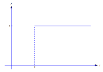
Thus, \(u(t)\) "steps" from the abiding value \(0\) to the constant value \(1\) at \(t=0\). If we replace \(t\) past \(t-\tau\) in Equation \ref{eq:8.four.iv}, and so
\[u(t-\tau)=\left\{\begin{assortment}{rl} 0,&t<\tau,\\ ane,&t\ge\tau \end{array}\right.; \nonumber\]
that is, the pace now occurs at \(t=\tau\) (Figure viii.iv.2 ).
The step office enables united states of america to represent piecewise continuous functions conveniently. For example, consider the role
\[\label{eq:8.four.5} f(t)=\left\{\begin{array}{rl} f_0(t),&0\le t<t_1,\\[4pt]f_1(t),&t\ge t_1, \terminate{array}\right.\]
where we assume that \(f_0\) and \(f_1\) are defined on \([0,\infty)\), fifty-fifty though they equal \(f\) only on the indicated intervals. This assumption enables u.s. to rewrite Equation \ref{eq:8.4.5} equally
\[\label{eq:8.iv.vi} f(t)=f_0(t)+u(t-t_1)\left(f_1(t)-f_0(t)\right).\]
To verify this, note that if \(t<t_1\) then \(u(t-t_1)=0\) and Equation \ref{eq:8.4.6} becomes
\[f(t)=f_0(t)+(0)\left(f_1(t)-f_0(t)\correct)=f_0(t). \nonumber\]
If \(t\ge t_1\) then \(u(t-t_1)=i\) and Equation \ref{eq:8.4.half dozen} becomes
\[f(t)=f_0(t)+(1)\left(f_1(t)-f_0(t)\right)=f_1(t). \nonumber\]
We need the side by side theorem to testify how Equation \ref{eq:8.4.vi} can be used to find \({\cal L}(f)\).
Allow \(thousand\) be defined on \([0,\infty).\) Suppose \(\tau\ge0\) and \({\cal L}\left(g(t+\tau)\right)\) exists for \(s>s_0.\) Then \({\cal L}\left(u(t-\tau)g(t)\right)\) exists for \(s>s_0\), and
\[{\cal 50}(u(t-\tau)g(t))=east^{-southward\tau}{\cal L}\left(k(t+\tau)\right).\nonumber\]
- Proof
-
By definition,
\[{\cal L}\left(u(t-\tau)g(t)\right)=\int_0^\infty e^{-st} u(t-\tau)chiliad(t)\, dt.\nonumber\]
From this and the definition of \(u(t-\tau)\),
\[{\cal 50}\left(u(t-\tau)g(t)\correct)=\int_0^\tau due east^{-st}(0)\,dt+\int_{\tau}^\infty e^{-st}g(t)\,dt.\nonumber\]
The first integral on the right equals cypher. Introducing the new variable of integration \(x=t-\tau\) in the second integral yields
\[{\cal L}\left(u(t-\tau)g(t)\right)=\int_0^\infty eastward^{-south(x+\tau)}1000(10+\tau)\,dx =e^{-southward\tau}\int_0^\infty due east^{-sx} g(x+\tau)\,dx.\nonumber\]
Changing the name of the variable of integration in the last integral from \(ten\) to \(t\) yields
\[{\cal L}\left(u(t-\tau)g(t)\right) =due east^{-s\tau}\int_0^\infty east^{-st} g(t+\tau)\,dt=e^{-s\tau}{\cal L}(g(t+\tau)).\nonumber\]
Find \[{\cal L}\left(u(t-1)(t^2+one)\correct).\nonumber\]
Solution
Hither \(\tau=1\) and \(g(t)=t^two+ane\), so
\[g(t+1)=(t+1)^ii+ane=t^2+2t+two.\nonumber\]
Since
\[{\cal L}\left(one thousand(t+ane)\right)={2\over s^3}+{2\over s^2}+{2\over s},\nonumber\]
Theorem viii.four.1 implies that
\[{\cal L}\left(u(t-i)(t^ii+ane)\right) =due east^{-due south}\left({2\over s^3}+{2\over s^2}+{ii\over south}\correct).\nonumber\]
Use Theorem 8.4.1 to find the Laplace transform of the part
\[f(t)=\left\{\brainstorm{array}{cl} 2t+one,&0\le t<2,\\[4pt]3t,&t\ge2, \end{array}\correct. \nonumber\]
from Instance 8.4.1 .
Solution
We first write \(f\) in the form Equation \ref{eq:eight.4.vi} equally
\[f(t)=2t+1+u(t-two)(t-1). \nonumber\]
Therefore
\[\brainstorm{aligned} {\cal 50}(f)&={\cal L}(2t+1) +{\cal Fifty}\left(u(t-ii)(t-1)\correct)\\ &={\cal L}(2t+1) +east^{-2s}{\cal L}(t+1)\quad\mbox{ (from Theorem }\PageIndex{1})\\ &={2\over s^2}+{ane\over s}+eastward^{-2s}\left({1\over south^2}+{1\over s}\correct),\stop{aligned}\nonumber\]
which is the result obtained in Instance viii.4.1 .
Formula Equation \ref{eq:viii.4.6} can be extended to more than full general piecewise continuous functions. For instance, we can write
\[f(t)=\left\{\brainstorm{assortment}{rl} f_0(t),&0\le t<t_1,\\[4pt]f_1(t),&t_1\le t<t_2,\\[4pt]f_2(t),&t\ge t_2, \finish{array}\right.\nonumber\]
as
\[f(t)=f_0(t)+u(t-t_1)\left(f_1(t)-f_0(t)\correct)+ u(t-t_2)\left(f_2(t)-f_1(t)\right) \nonumber\]
if \(f_0\), \(f_1\), and \(f_2\) are all defined on \([0,\infty)\).
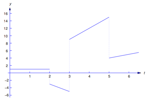
Notice the Laplace transform of
\[\label{eq:8.4.7} f(t)=\left\{\begin{assortment}{cl} 1,&0\le t<2,\\[4pt]-2t+1,&2\le t<3,\\[4pt]3t,&3\le t<5,\\[4pt]t-one,&t\ge5 \cease{array}\correct.\]
(Figure eight.4.3 ).
Solution
In terms of step functions,
\[\begin{aligned} f(t)&=1+u(t-2)(-2t+1-1)+u(t-3)(3t+2t-1)\\ &= +u(t-five)(t-1-3t),\end{aligned}\nonumber\]
or
\[f(t)=1-2u(t-2)t+u(t-3)(5t-one)-u(t-five)(2t+one). \nonumber\]
Now Theorem eight.4.1 implies that
\[\begin{aligned} {\cal L}(f)&={\cal L}(one)-2e^{-2s}{\cal L}(t+two)+e^{-3s}{\cal Fifty}\left(5(t+3)-1\right)-e^{-5s}{\cal L}\left(2(t+5)+1\correct)\\[4pt]&={\cal 50}(one)-2e^{-2s}{\cal L}(t+2)+e^{-3s}{\cal L}(5t+xiv)-e^{-5s}{\cal L}(2t+11)\\[4pt]&={one\over s}-2e^{-2s}\left({i\over s^2}+{2\over due south}\right)+ e^{-3s}\left({5\over south^2}+{14\over s}\right)-e^{-5s}\left({ii\over south^2}+{11\over s}\correct). \stop{aligned}\nonumber\]
The trigonometric identities
\[\label{eq:8.4.8} \sin (A+B)=\sin A\cos B+\cos A\sin B\]
\[\label{eq:8.iv.ix} \cos (A+B)=\cos A\cos B-\sin A\sin B\]
are useful in issues that involve shifting the arguments of trigonometric functions. We'll utilize these identities in the adjacent example.
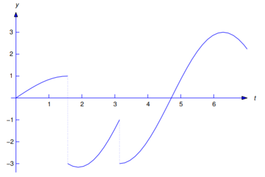
Find the Laplace transform of
\[\label{eq:8.iv.10} f(t)=\left\{\begin{array}{cl}{\sin t,}&{0\leq t<\frac{\pi }{ii}}\\{\cos t-3\sin t,}&{\frac{\pi }{ii}\leq t<\pi }\\{3\cos t,}&{t\geq \pi} \end{array} \right.\]
(Figure viii.iv.four ).
Solution
In terms of step functions,
\[f(t)=\sin t+u(t-\pi/2) (\cos t-4\sin t)+u(t-\pi) (2 \cos t+3\sin t). \nonumber\]
At present Theorem 8.4.1 implies that
\[\label{eq:8.four.eleven} \begin{array}{ccl} {\cal L}(f)&=&{\cal L}(\sin t)+e^{-{\pi\over ii}s}{\cal Fifty} \left(\cos\left(t+{\pi\over2}\right)-four\sin\left(t+{\pi\over2}\right)\right) \\[4pt]&&\qquad+e^{-\pi s}{\cal L}\left(2\cos(t+\pi)+three\sin(t+\pi)\right). \cease{array}\]
Since
\[\cos\left(t+{\pi\over ii}\right)-iv\sin\left(t+{\pi\over ii}\right)=-\sin t-four\cos t \nonumber\]
and
\[ii\cos (t+\pi)+3\sin (t+\pi)=-2\cos t-3\sin t, \nonumber\]
we meet from Equation \ref{eq:8.4.xi} that
\[\brainstorm{marshal*} {\cal L}(f)&={\cal L}(\sin t)-e^{-\pi s/ii}{\cal Fifty}(\sin t+iv\cos t) -e^{-\pi south}{\cal L}(2\cos t+3\sin t)\\[4pt]&={1\over s^two+i}-east^{-{\pi\over two}s}\left({1+4s\over s^2+i}\right) -e^{-\pi s}\left({3+2s\over s^two+one}\right). \stop{align*}\nonumber\]
The Second Shifting Theorem
Replacing \(g(t)\) by \(g(t-\tau)\) in Theorem 8.4.1 yields the next theorem.
If \(\tau\ge0\) and \({\cal L}(g)\) exists for \(s>s_0\) and then \({\cal L}\left(u(t-\tau)m(t-\tau)\right)\) exists for \(south>s_0\) and
\[{\cal L}(u(t-\tau)g(t-\tau))=eastward^{-southward\tau}{\cal L}(grand(t)),\nonumber\]
or, equivalently,
\[\label{eq:8.4.12} \mbox{if } g(t)\leftrightarrow One thousand(s),\mbox{ and so }u(t-\tau)one thousand(t-\tau)\leftrightarrow due east^{-s\tau}G(s).\]
Recollect that the First Shifting Theorem (Theorem 8.1.iii states that multiplying a function by \(east^{at}\) corresponds to shifting the argument of its transform past a units. Theorem 8.4.2 states that multiplying a Laplace transform past the exponential \(eastward^{−\tau due south}\) corresponds to shifting the statement of the changed transform past \(\tau \) units.
Apply Equation \ref{eq:8.4.12} to find
\[{\cal 50}^{-1}\left(e^{-2s}\over s^ii\right). \nonumber\]
Solution
To use Equation \ref{eq:viii.4.12} nosotros allow \(\tau=2\) and \(G(due south)=1/due south^2\). Then \(g(t)=t\) and Equation \ref{eq:8.4.12} implies that
\[{\cal L}^{-1}\left(e^{-2s}\over s^2\right)=u(t-two)(t-ii).\nonumber\]
Find the inverse Laplace transform \(h\) of
\[H(due south)={one\over s^2}-e^{-s}\left({i\over s^2}+{2\over south}\correct)+ e^{-4s}\left({4\over s^three}+{1\over s}\right),\nonumber\]
and notice distinct formulas for \(h\) on appropriate intervals.
Solution
Permit
\[G_0(s)={one\over southward^two},\quad G_1(south)={1\over s^2}+{2\over s},\quad G_2(s)={4\over due south^3}+{one\over s}.\nonumber\]
And so
\[g_0(t)=t,\; g_1(t)=t+2,\; g_2(t)=2t^2+1.\nonumber\]
Hence, Equation \ref{eq:8.4.12} and the linearity of \({\cal L}^{-1}\) imply that
\[\begin{aligned} h(t)&={\cal Fifty}^{-1}\left(G_0(s)\right)-{\cal L}^{-1}\left(e^{-s}G_1(s)\right)+{\cal L}^{-1}\left(eastward^{-4s}G_2(south)\right)\\[4pt]&=t-u(t-1)\left[(t-i)+2\right]+u(t-4)\left[2(t-four)^2+one\right]\\[4pt]&=t-u(t-1)(t+1)+u(t-4)(2t^ii-16t+33),\terminate{aligned}\nonumber\]
which tin can also exist written equally
\[h(t)=\left\{\begin{array}{cl} t,&0\le t<1,\\[4pt]-ane,&1\le t<4,\\[4pt]2t^2-16t+32,&t\ge4. \end{array}\right.\nonumber \]
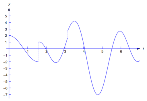
Find the inverse transform of
\[H(southward)={2s\over due south^2+4}-eastward^{-{\pi\over 2}s} {3s+one\over southward^2+nine}+e^{-\pi s}{due south+1\over south^two+6s+10}. \nonumber\]
Solution
Permit
\[G_0(s)={2s\over s^two+4},\quad G_1(south)=-{(3s+1)\over s^2+9},\nonumber\]
and
\[G_2(southward)={s+ane\over s^2+6s+10}={(s+3)-2\over (s+3)^2+1}.\nonumber\]
Then
\[g_0(t)=two\cos 2t,\quad g_1(t)=-3\cos 3t-{1\over 3}\sin 3t,\nonumber\]
and
\[g_2(t)=due east^{-3t}(\cos t-2\sin t).\nonumber\]
Therefore Equation \ref{eq:viii.4.12} and the linearity of \({\cal Fifty}^{-one}\) imply that
\[\begin{aligned} h(t)&=ii\cos 2t-u(t-\pi/2)\left[3\cos 3(t-\pi/2)+{1\over three}\sin three\left(t-{\pi\over two}\right)\right]\\[4pt] &= +u(t-\pi)e^{-three(t-\pi)}\left[\cos (t-\pi)-2\sin (t-\pi)\right].\terminate{aligned}\nonumber\]
Using the trigonometric identities Equation \ref{eq:eight.4.viii} and Equation \ref{eq:8.iv.9}, nosotros can rewrite this as
\[\characterization{eq:8.iv.13} \begin{marshal} h(t)&=2\cos 2t+u(t-\pi/2)\left(3\sin 3t- {1\over 3}\cos 3t\right) \\[4pt] &= -u(t-\pi)e^{-3(t-\pi)} (\cos t-2\sin t) \end{align}\]
(Figure 8.4.v ).

Unit Step Function Laplace Transform,
Source: https://math.libretexts.org/Bookshelves/Differential_Equations/Book:_Elementary_Differential_Equations_with_Boundary_Value_Problems_%28Trench%29/08:_Laplace_Transforms/8.04:_The_Unit_Step_Function
Posted by: cravenalling69.blogspot.com
0 Response to "Unit Step Function Laplace Transform"
Post a Comment